

Let's work together!
Like my work? I'm happy to connect.
During a reconnaissance mission gone wrong, R2-D2 was attacked by Stormtroopers, leaving his executive control unit disconnected from his motor control unit. We need to help him by SSHing into his motor control unit and guiding him to the rendezvous with C-3PO and Luke. The environment is a maze riddled with obstacles, and time is of the essence. Below, you can see how we were able to program and run the A* search algorithm (among others), integrate motor controls via R2D2's motor control unit API, and use Augmented Reality (AR) to interact between a 3D world and 2D image to help R2D2 get to safety.
In order to solve a maze, we first need to create a representation of a maze that we can use for the search algorithms. We implement our maze as a graph, where each vertex represents a grid cell, and an edge between vertices represents the ability to traverse between those grid cells. The graph is directed and unweighted, with its edges stored as an adjacency list. The initialization of Graph(V, E) takes in a set of vertices V = {v_1, v_2, ...} and a set of edges E = {(v_1, v_2), (v_3, v_4), ...}.
Breadth First Search (BFS) returns the shortest path
from the start to the goal.
Breadth-first search starts from a selected node
and explores all of the neighbor nodes
at the present depth / on the same level before moving on
to the nodes at the next level of depth.
In other words, BFS explores vertices in the order of
their distance from the source vertex,
where distance is the minimum length of a path
from the source vertex to the node.
Breadth-first search can be implemented
using a queue data structure,
which follows the first-in-first-out (FIFO) method
– i.e., the node that was inserted first
will be visited first.
def bfs(
    self, start: Vertex, goal: Vertex
) -> Tuple[Optional[List[Vertex]], Set[Vertex]]:
    """
    Use BFS algorithm to find the path from start to goal
    in the given graph.

    :return:  a tuple (shortest_path, node_visited),
              where shortest_path is a list of vertices
              that represents the path from start to goal,
              and None if such a path does not exist;
              node_visited is a set of vertices
              that are visited during the search.
    """
    if start not in self.vertices or goal not in self.vertices:
        return (None, None)

    node_visited = {start}
    shortest_path = []
    parents = {start: None}

    if start == goal:
        return (shortest_path, node_visited)

    queue = [start]
    while len(queue) > 0:
        current_vertex = queue.pop(0)

        if current_vertex == goal:
            # backtrack through parents to get path
            shortest_path = [goal]
            temp = current_vertex
            while parents[temp] != None:
                shortest_path.insert(0, parents[temp])
                temp = parents[temp]
            return (shortest_path, node_visited)

        neighbors = self.neighbors(current_vertex)
        for neighbor in neighbors:
            if neighbor not in node_visited:
                queue.append(neighbor)
                parents[neighbor] = current_vertex
                node_visited.add(neighbor)

    return (None, None)
DFS does not necessarily return the shortest path,
but as a benefit, it generally requires less memory
compared to other search algorithms (ex. BFS)
because it uses a stack data structure.
DFS follows the last-in-first-out (LIFO) method – i.e.,
the node that was inserted last will be visited first.
That is, DFS explores the highest-depth nodes first
before backtracking and expanding shallower nodes.
We use a recursive Depth First Search (DFS) implementation:
def dfs(
    self, start: Vertex, goal: Vertex
) -> Tuple[Optional[List[Vertex]], Set[Vertex]]:
    """
    Use DFS algorithm to find the path from start to goal
    in the given graph.

    :return:  a tuple (valid_path, node_visited),
              where valid_path is a list of vertices
              that represents the path from start to goal
              (no need to be shortest),
              and None if such a path does not exist;
              node_visited is a set of vertices
              that are visited during the search.
    """
    if start not in self.vertices or goal not in self.vertices:
        return (None, None)

    visited = set()

    def dfs_visit(node):
          if node in visited:
                return None
          visited.add(node)
          if node == goal:
                return [goal]
          for neighbor in self.neighbors(node):
                res = dfs_visit(neighbor)
                if res:
                      res.append(node)
                      return res

    valid_path = dfs_visit(start)
    valid_path.reverse()

    return valid_path, visited
A* is an informed search algorithm,
or a best-first search, meaning that
starting from a specific starting node of a graph,
it aims to find a path to the given goal node
having the smallest cost (we're looking for shortest distance).
The key idea is that we avoid expanding paths
that have a high cost, and instead pursue paths
that have a low estimated cost.
At each iteration of its main loop,
A* needs to determine which of its paths to extend.
It does so based on the cost of the path
and an estimate of the cost required to extend the path
all the way to the goal.
Specifically, A* selects the path that minimizes
f(n)=g(n)+h(n) where n
is the next node on the path, g(n)
is the cost of the path from the start node to n,
and h(n) is a heuristic function
that estimates the cost of the lowest-cost path
from n to the goal.
If the heuristic function is admissible
– meaning that it never overestimates the actual cost
to get to the goal –,
A* is guaranteed to return a least-cost path
from start to goal.
A* terminates when the path it chooses to extend
is a path from start to goal,
or if there are no paths eligible to be extended.
def a_star(
    self, start: Vertex, goal: Vertex
) -> Tuple[Optional[List[Vertex]], Set[Vertex]]:
    """
    Use A* algorithm to find the path from start to goal
    in the given graph.

    :return:  a tuple (shortest_path, node_visited),
              where shortest_path is a list of vertices
              that represents the path from start to goal,
              and None if such a path does not exist;
              node_visited is a set of vertices
              that are visited during the search.
    """
    parent = {start: None}
    # best_so_far = dict, shortest encountered path distance to a node
    best_so_far = {start: 0}
    # for node n: n[0] = x-coordinate, n[1]= y coorodinate
    heuristic = lambda n: abs(n[0] - goal[0]) + abs(n[1] - goal[1])
    # [(heuristic value of node, cumulative distance of node, node)]
    heap = [(heuristic(start), 0, start)]

    while len(heap) > 0:
        _, cuml_distance, node = heapq.heappop(heap)
        if best_so_far[node] < cuml_distance:
            continue
        if node == goal:
            # backtrack through parents to get path
            return self._backtrace(parent, goal), set(parent.keys())

        neighbor_cuml_distance = cuml_distance + 1
        for neighbor_node in self.neighbors(node):
            if neighbor_cuml_distance < best_so_far.get(neighbor_node, float("inf")):
                heapq.heappush(
                    heap,
                    (
                        neighbor_cuml_distance + heuristic(neighbor_node),
                        neighbor_cuml_distance,
                        neighbor_node,
                    ),
                )
                best_so_far[neighbor_node] = neighbor_cuml_distance
                parent[neighbor_node] = node
The Traveling Sales Person (TSP) problem requires
solving a search problem with multiple goals.
The tsp method returns the shortest path which visits all of the
goal nodes, beginning with the start node.
The implementation generates permutations of
the target nodes and uses A* to calculate
the shortest path between the nodes.
It then identifies the optimal order which has the shortest total path.
def tsp(
    self, start: Vertex, goals: Set[Vertex]
) -> Tuple[Optional[List[Vertex]], Optional[List[Vertex]]]:
    """
    Use A* algorithm to find the path that begins at start
    and passes through all the goals in the given graph,
    in an order such that the path is the shortest.

    :return:  a tuple (optimal_order, shortest_path),
              where shortest_path is a list of vertices
              that represents the path from start that
              goes through all the goals such that the path is the shortest;
              optimal_order is an ordering of goals that is visited
              in the order that results in the above shortest_path.
              Return (None, None) if no such path exists.
    """
    shortest_length = float("inf")
    optimal_order = None
    shortest_path = None
    for ordered_goals in permutations(goals):
        paths = [start]
        prev = start
        for goal in ordered_goals:
            path, _ = self.a_star(prev, goal)
            paths += path[1:]
            prev = goal
        if len(paths) < shortest_length:
            shortest_length = len(paths)
            shortest_path = paths
            optimal_order = ordered_goals
    return optimal_order, shortest_path
The GUI visualizes the performance of the search algorithms. Note that later on this will be translated to 3D. To start the GUI with a maze of specific dimensions and random obstacles, you can use:
python3 gui.py {number of rows} {number of columns}
If you don’t add any parameters when running the GUI, then the GUI uses the custom map defined in the custom_map method.
It should be noticed that the green triangles represent the direction of the edges between the vertices if there is only one directed edge between the cells.
When running, left-click on the grid squares to select the start point and right-click to select the goal point for the search. For tsp search, you can select multiple goal points. The drop-down menu on the right side enables the user to choose which algorithm to use, and the "Find Path" button runs the search and displays the path solution. The light blue squares denote the nodes visited during the searching process. The "Clear Paths" button makes it easy to start again.
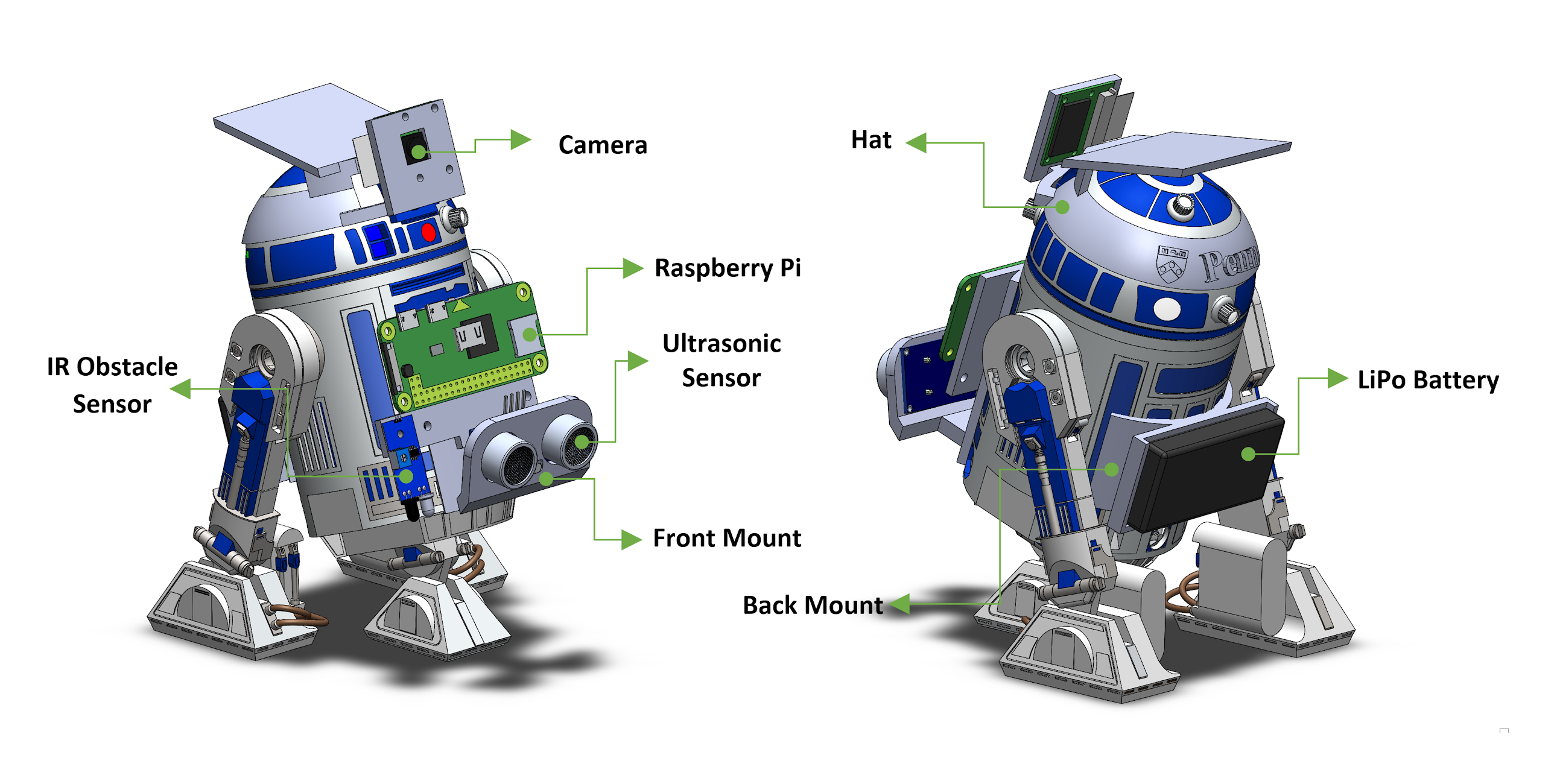
Now it’s time for R2-D2 to show off the path planning skills in real world. We use a Sphero R2D2 robot equipped with Raspberry Pi, sensors, and a camera system.
The basic Sphero R2D2 does not have many built in sensors. We upgraded the droid with a sensor pack attached to the robot via a 3D printed mount. We add an ultrasonic sensor range finder, an IR cliff sensor, and a camera.
The ultrasonic sensor uses sound waves to measure the distance to obstacles. Here, the ultrasonic sensor is mounted on the front armor with glue to detect the obstacles in front of the R2-D2.
Instead of utilizing sound waves, the infrared transmitter (IR) obstacle sensor uses light radiation to perceive the obstacles. The IR sensor is linked to the front mount using screws and points to the ground to detect cliffs.
The camera is mounted on the hat mount with screws which can be easily dismounted. The camera has a resolution of 1080p/30fps.
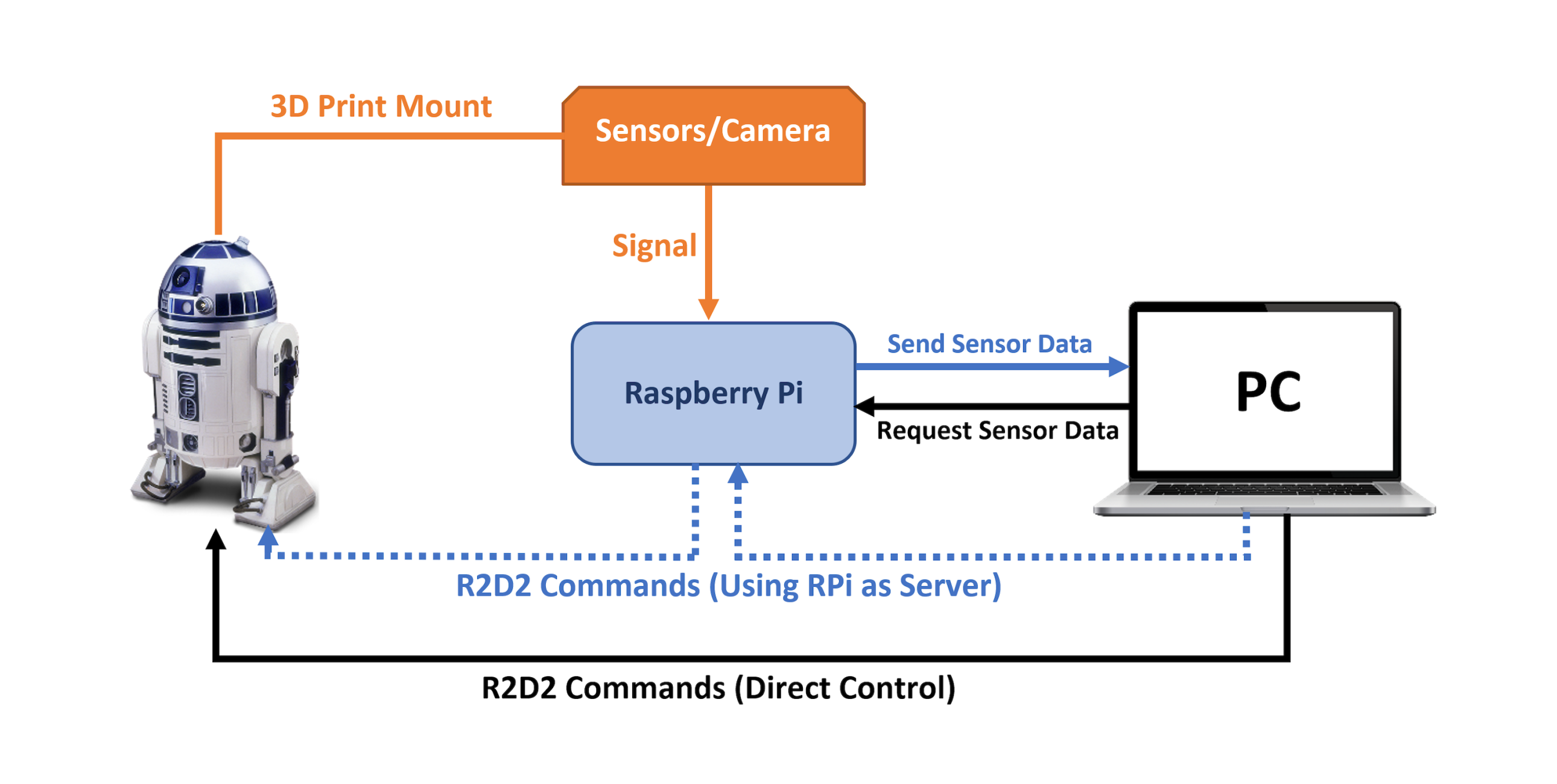
Now, R2-D2 can take advantage of its new sensors and camera to act rationally. In this part, the R2-D2 uses the ultrasonic sensor and the IR obstacle sensor to perceive the environment and make decisions based on the sensor data.
The Sphero API provides an on_collision event which can detect whether the R2-D2 has hit something or not by using its built-in accelerometer. However, the built-in sensor only reports an obstacle when the droid collides with it. The ultrasonic sensor, on the other hand, uses the time that the ultrasound takes to get reflected off of an object to estimate the distance to the target.
To prevent collisions, the R2-D2 uses the ultrasonic sensor to detect the distance to any obstacles and act rationally based on the feedback. obstacle_avoidance() allows the R2-D2 to stop and turn after detecting an obstacle. We follow the following logic:
Every 0.1 seconds, check for obstacles.
We can see the performance of the droid in the simulation and of R2D2:
Now we create an Augmented Reality (AR) Environment for R2D2.
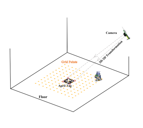
In order to implement the AR application, we must have a way to interact between 3D world and 2D image. A widely used approach is using a transformation matrix which defines the relationship between a real-world coordinate and an image coordinate.
Given the coordinate of a 3D point in real world, we use a transformation matrix P to calculate its 2D image coordinate.
The transformation matrix P=K[R|T] consists of rotation R (roll, pitch, yaw), translation T between the two coordinate systems, and K, the intrinsic matrix of the camera.
Once we have calculated the transformation matrix P, we convert points in the real world to the image points using the equation x=PX.
AprilTag is a visual fiducial system that looks like a QR code which is useful for a wide variety of tasks including augmented reality (AR), robotics, and camera calibration. You can understand how it works from this paper.
We use AprilTag to compute the rotation R and translation matrices T between the world coordinate and the camera coordinate (the Detector package from the library pupil_apriltags gives us these matrices). Then, we use the two matrices to get the transformation matrix P. Now, for any point in the real world, we can compute its image coordinate based on the transformation matrix x=PX.
We use the following methods:
Now, we can use the real time AR in a room. First, we put the AprilTag on the floor and keep it flat. Next, with Raspberry Pi and the camera running, we use:
python3 ar_maze.py
to launch a video streaming window showing the grid. Just an in the GUI shown previously, we can select start and end goals. We can also define and un-define obstacles, and calculate a path using one of search algorithms implemented earlier.
With a path identified, R2D2 uses the following to reach the goal:
R2-D2 should be placed at the center of the starting point chosen in the AR maze (make sure it is heading the same direction with the AprilTag). With this done, we can execute the path using the robot. Awesome!
Access to private GitHub repository can be provided upon request.
Like my work? I'm happy to connect.